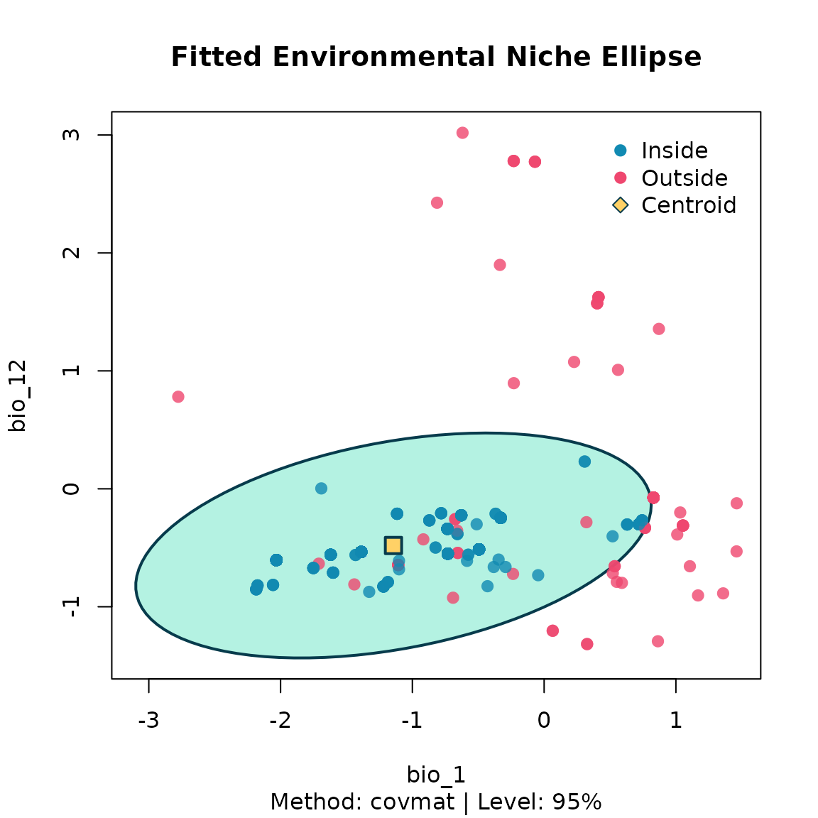
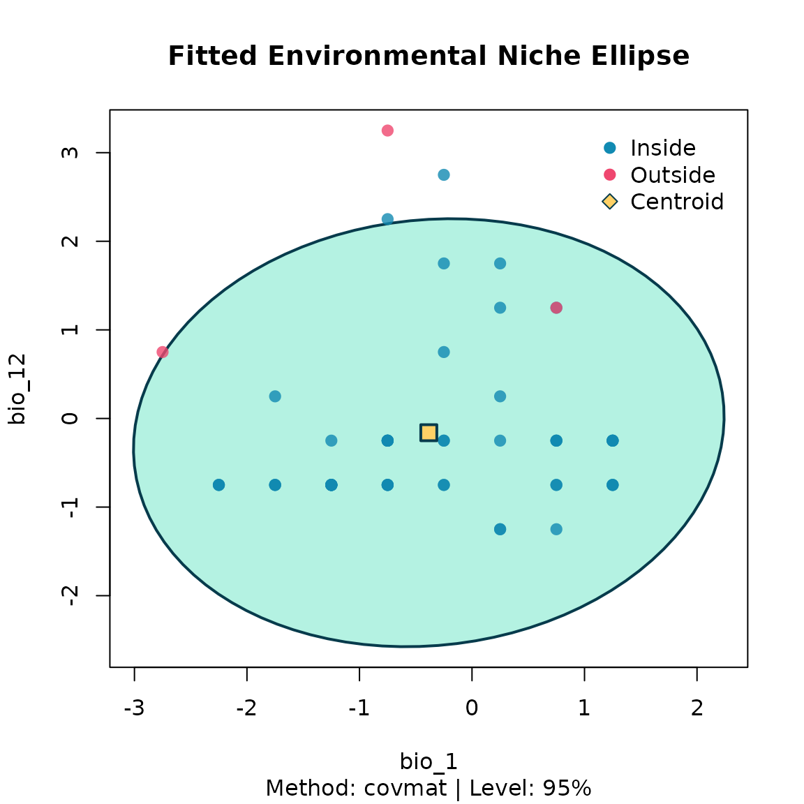
After thinning, the environmental niche is summarised by a
multivariate ellipsoid via fit_ellipsoid(). Two estimators
are available:
-
"covmat"— classical sample mean and covariance. -
"mve"— robust Minimum Volume Ellipsoid (Rousseeuw, 1985).
The ellipsoid boundary is defined by a chi-square cutoff on the
squared Mahalanobis distance, controlled by level (default
95 %).
library(bean)
data(origin_dat_prepared, package = "bean")
data(thinned_stochastic, package = "bean")
data(thinned_deterministic, package = "bean")
env_vars <- c("bio_1", "bio_4", "bio_12", "bio_15")
Fit three ellipsoids
We fit one ellipsoid to the raw prepared data and one to each of the thinned datasets, so we can compare what bias correction does to the inferred niche.
origin_ellipse <- fit_ellipsoid(
  data = origin_dat_prepared,
  env_vars = env_vars,
  method = "covmat",
  level = 0.95
)

stochastic_ellipse <- fit_ellipsoid(
  data = thinned_stochastic$thinned_data,
  env_vars = env_vars,
  method = "covmat",
  level = 0.95
)

deterministic_ellipse <- fit_ellipsoid(
  data = thinned_deterministic$thinned_points,
  env_vars = env_vars,
  method = "covmat",
  level = 0.95
)

origin_ellipse
#> -- Bean Environmental Niche Ellipsoid --
#> Method      : covmat
#> Dimensions  : 4 (bio_1, bio_4, bio_12, bio_15)
#> Level       : 95.00%
#> Points used : 1024  (inside: 947, 92.5%)
#> Centroid:
#>      bio_1      bio_4     bio_12     bio_15
#> -1.1433128 -0.1851743 -0.4804313 -0.4194209
stochastic_ellipse
#> -- Bean Environmental Niche Ellipsoid --
#> Method      : covmat
#> Dimensions  : 4 (bio_1, bio_4, bio_12, bio_15)
#> Level       : 95.00%
#> Points used : 78  (inside: 71, 91.0%)
#> Centroid:
#>      bio_1      bio_4     bio_12     bio_15
#> -0.3502912 -0.3690432 -0.1938518 -0.4200464
deterministic_ellipse
#> -- Bean Environmental Niche Ellipsoid --
#> Method      : covmat
#> Dimensions  : 4 (bio_1, bio_4, bio_12, bio_15)
#> Level       : 95.00%
#> Points used : 56  (inside: 53, 94.6%)
#> Centroid:
#>      bio_1      bio_4     bio_12     bio_15
#> -0.3839286 -0.4732143 -0.1607143 -0.4464286
Visualise the ellipsoids (2-D slices)

For an interactive 3-D view, install the optional package
rgl and call
plot(origin_ellipse, dims = c(1, 2, 3)). If
rgl is not installed, the plot falls back to the 2-D view
of the first two requested variables.
Inspecting the inferred niche
fit_ellipsoid() returns an object that exposes the
centroid, the covariance matrix, the precomputed inverse, the variable
names, and the subset of points classified as inside or outside the
ellipsoid. These are the building blocks downstream
species-distribution-modelling pipelines need.
origin_ellipse$centroid
#>      bio_1      bio_4     bio_12     bio_15
#> -1.1433128 -0.1851743 -0.4804313 -0.4194209
origin_ellipse$cov_matrix
#>              bio_1       bio_4      bio_12      bio_15
#> bio_1   0.63868536 -0.08168806  0.11201568  0.01955072
#> bio_4  -0.08168806  0.11787467 -0.08758222  0.05482355
#> bio_12  0.11201568 -0.08758222  0.15183243 -0.06084654
#> bio_15  0.01955072  0.05482355 -0.06084654  0.07808037
origin_ellipse$dimensions
#> [1] 4
origin_ellipse$var_names
#> [1] "bio_1"  "bio_4"  "bio_12" "bio_15"
head(origin_ellipse$points_in_ellipse)
#>         species        y         x      bio_1       bio_12     bio_15
#> 1 Rusa unicolor 15.37239  99.11555 -1.6909295  0.003511156 -0.2454693
#> 2 Rusa unicolor 15.41415  99.28763 -0.8711075 -0.267821213 -0.3053829
#> 3 Rusa unicolor 14.46838 101.22005 -1.3879976 -0.534812263 -0.3835742
#> 4 Rusa unicolor 15.65606  99.31600 -0.6288324 -0.224408034 -0.2390396
#> 5 Rusa unicolor 14.39543 101.41694 -2.0311866 -0.604273349 -0.5074636
#> 7 Rusa unicolor 14.40847 101.29556 -1.3879976 -0.534812263 -0.3835742
#>        bio_4
#> 1 -0.2573387
#> 2 -0.1768698
#> 3 -0.2876102
#> 4 -0.0834852
#> 5 -0.1398570
#> 7 -0.2876102
Projecting suitability with nicheR
If you intend to project a bean_ellipsoid into
geographic space, please install the nicheR package and
use its predict() method. bean_ellipsoid
objects carry "nicheR_ellipsoid" as a second S3 class, so
once nicheR is attached its predict.nicheR_ellipsoid()
method dispatches on them automatically — no conversion step is
required. If you use the prediction step in published work, please cite
nicheR (see the References section at the bottom of this vignette).
Installing and loading nicheR
nicheR is available on CRAN:
install.packages("nicheR")
library(nicheR)
Predicting suitability
When both nicheR and terra are available, the chunk below runs the prediction for all three ellipsoids and plots the suitability layers side by side. When either package is missing, the chunk is skipped automatically.
The ellipsoids were fitted on the scaled environmental variables in
origin_dat_prepared (the output of
prepare_bean(transform = "scale")). The raster must be
scaled the same way before being passed to predict(),
otherwise the Mahalanobis distances would be computed in a different
coordinate system from the one in which the ellipsoid was defined. We
use terra::scale() to apply standardisation layer by
layer.
library(nicheR)
library(terra)
#> terra 1.9.27

# Load the raster and scale each layer to mean 0, SD 1 — matching how
# the ellipsoids were trained.
env <- terra::rast(system.file("extdata", "thai_env.tif",
                               package = "bean"))
env_scaled <- terra::scale(env)

# Project each ellipsoid back into geographic space.
origin_suit <- predict(
  origin_ellipse,
  newdata             = env_scaled,
  include_suitability = TRUE,
  include_mahalanobis = FALSE
)
#> Starting: suitability prediction using newdata of class: SpatRaster...
#> Step: Using 4 predictor variables: bio_1, bio_4, bio_12, bio_15
#> Done: Prediction completed successfully. Returned raster layers: suitability

stochastic_suit <- predict(
  stochastic_ellipse,
  newdata             = env_scaled,
  include_suitability = TRUE,
  include_mahalanobis = FALSE
)
#> Starting: suitability prediction using newdata of class: SpatRaster...
#> Step: Using 4 predictor variables: bio_1, bio_4, bio_12, bio_15
#> Done: Prediction completed successfully. Returned raster layers: suitability

deterministic_suit <- predict(
  deterministic_ellipse,
  newdata             = env_scaled,
  include_suitability = TRUE,
  include_mahalanobis = FALSE
)
#> Starting: suitability prediction using newdata of class: SpatRaster...
#> Step: Using 4 predictor variables: bio_1, bio_4, bio_12, bio_15
#> Done: Prediction completed successfully. Returned raster layers: suitability

# Three-panel comparison: Original / Stochastic / Deterministic.
# A shared colour scale (range = [0, 1]) makes the panels directly
# comparable; the same legend applies to all three.
op <- par(mfrow = c(1, 3), mar = c(2.5, 2.5, 3, 4))
terra::plot(origin_suit[["suitability"]],
            main  = "Original (unthinned)",
            range = c(0, 1))
terra::plot(stochastic_suit[["suitability"]],
            main  = "Stochastic thinning",
            range = c(0, 1))
terra::plot(deterministic_suit[["suitability"]],
            main  = "Deterministic thinning",
            range = c(0, 1))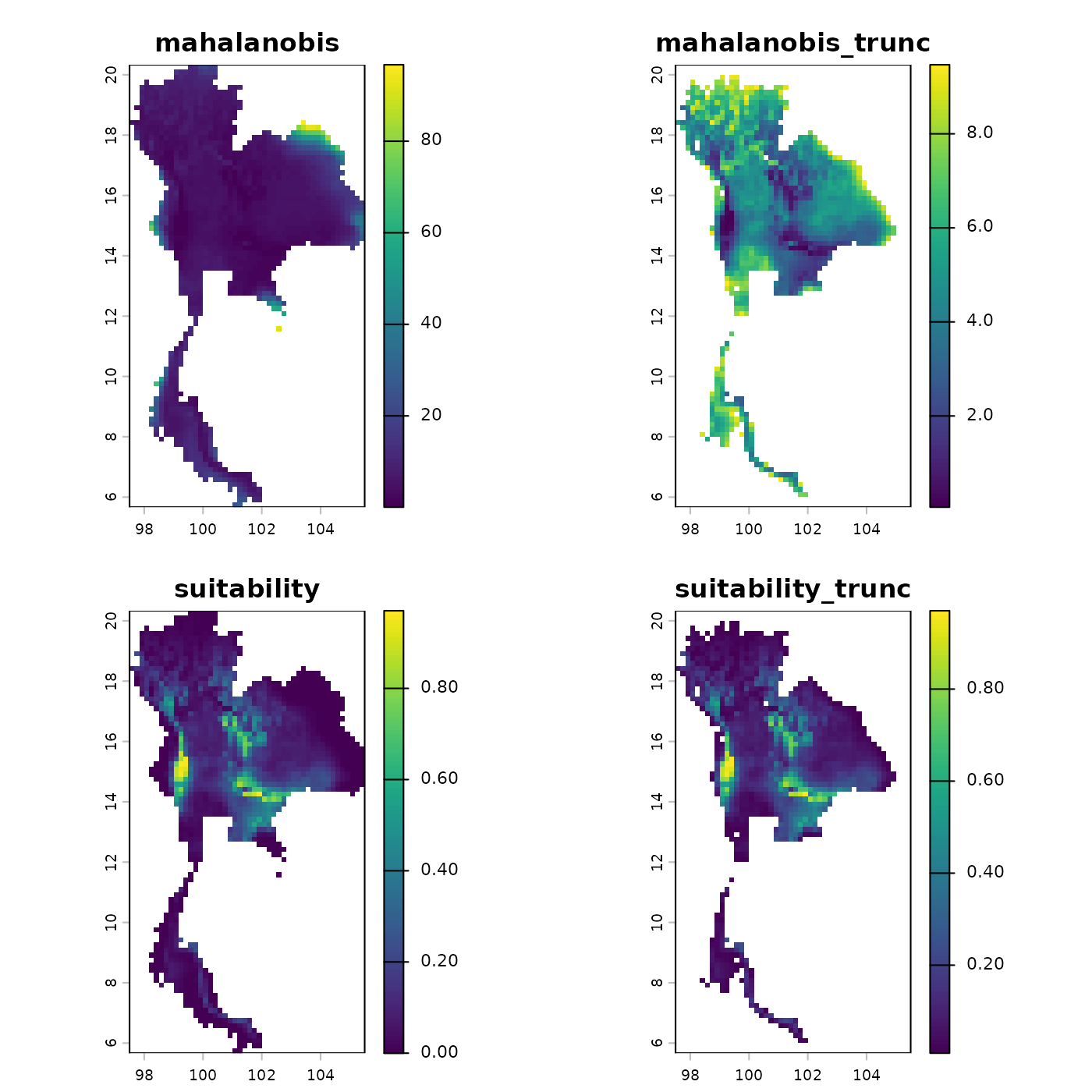
par(op)Because the raw data is biased toward heavily sampled environments, the unthinned model typically over-predicts those conditions. Both thinned models produce a narrower, less inflated suitability surface — the expected effect of bias correction.
References
- Castaneda-Guzman, M., Hughes, C., Paansri, P., & Cobos, M. E. (2026). nicheR: Ellipsoid-Based Virtual Niches and Visualization. R package version 0.1.0. https://github.com/castanedaM/nicheR
- Rousseeuw, P. J. (1985). Multivariate estimation with high breakdown point. Mathematical Statistics and Applications, Vol. B, 283–297.
- Van Aelst, S. & Rousseeuw, P. (2009). Minimum volume ellipsoid. Wiley Interdisciplinary Reviews: Computational Statistics, 1(1), 71–82.