Find an objective environmental grid resolution

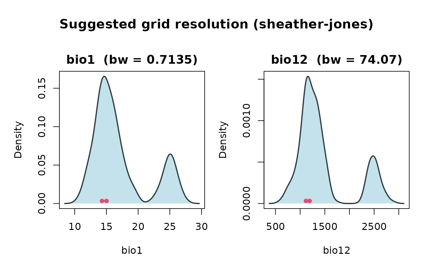
Calculates an objective, data-driven grid resolution for environmental thinning. For each environmental variable, the function selects a bandwidth for a kernel-density estimate (KDE) of the marginal distribution. The chosen bandwidth defines the spatial scale below which two observations carry essentially redundant information, and is therefore a natural choice for the edge length of an environmental grid cell.

Three established bandwidth selectors are supported (see Details):

"sheather-jones" (default) — the Sheather–Jones direct plug-in estimator (Sheather & Jones, 1991), the modern recommended default for non-Gaussian data;
"silverman" — Silverman's rule of thumb (Silverman, 1986);
"scott" — Scott's rule (Scott, 1992).

Usage

find_env_resolution(
  data,
  env_vars,
  method = c("sheather-jones", "silverman", "scott")
)

Arguments

data: A data.frame containing the environmental variables.
env_vars: A character vector specifying the environmental variables to analyse.
method: The bandwidth selector. One of "sheather-jones" (default), "silverman", or "scott".

Value

An object of class bean_env_resolution (a list) with:

suggested_resolution: A named numeric vector of the suggested grid resolution for each variable, in the units of that variable.
bandwidths: The bandwidths used to derive each resolution (identical to suggested_resolution).
density_data: A long-format data.frame of the kernel density estimates, used by plot.bean_env_resolution.
method: The bandwidth selector that was used.

Details

Why a bandwidth? A good environmental grid cell should be small enough to distinguish ecologically meaningful differences, but large enough to absorb sampling noise. A kernel density bandwidth chosen from the data answers exactly that question: it is the scale at which the empirical density of observations becomes smooth. Using it as the grid resolution yields one occurrence per cell on average when the sampling intensity is near the mode of the data.

Selectors.

Sheather–Jones (stats::bw.SJ with method = "dpi") is a plug-in selector that is robust for non-Gaussian densities and is the standard recommendation in the modern literature (Sheather & Jones, 1991; Jones, Marron & Sheather, 1996). Recommended default.
Silverman (stats::bw.nrd0) is the rule-of-thumb \(h = 0.9 \, \min(\hat\sigma, IQR/1.34) \, n^{-1/5}\) (Silverman, 1986). Fast and stable, but assumes near-Gaussian shape.
Scott (stats::bw.nrd) is the Gaussian-optimal rule \(h = 1.06 \, \hat\sigma \, n^{-1/5}\) (Scott, 1992). Simpler than Silverman but less robust to outliers.

If "sheather-jones" fails (this can happen with strongly tied data), the function falls back to Silverman's rule for that variable and emits a message().

References

Sheather, S. J. & Jones, M. C. (1991). A reliable data-based bandwidth selection method for kernel density estimation. Journal of the Royal Statistical Society: Series B, 53(3), 683–690.

Silverman, B. W. (1986). Density Estimation for Statistics and Data Analysis. Chapman & Hall, London.

Scott, D. W. (1992). Multivariate Density Estimation: Theory, Practice, and Visualization. Wiley, New York.

Jones, M. C., Marron, J. S. & Sheather, S. J. (1996). A brief survey of bandwidth selection for density estimation. Journal of the American Statistical Association, 91(433), 401–407.

Examples

set.seed(1)
df <- data.frame(
  bio1  = c(rnorm(200, 15, 2), rnorm(50, 25, 1)),
  bio12 = c(rnorm(200, 1200, 200), rnorm(50, 2500, 100))
)
res <- find_env_resolution(df, env_vars = c("bio1", "bio12"))
res$suggested_resolution
#>       bio1      bio12 
#>  0.7134594 74.0651811 
plot(res)